5. Inferencing with DeepH
In this part, we demonstrate quick examples for DeepH inference.
Note
This chapter should be done in the deeph environment.
5.1. Prepare Dataset for Inference
The overlap matrix plays a dual yet distinct role in DeepH workflows. While its structural sparsity pattern is indispensable for constructing the atomic connectivity graph during training (though the specific matrix values do not affect model optimization), the actual numerical values become essential only for post-inference diagonalization when calculating band structures.
Crucially, generating this structural information requires minimal computational overhead: By setting sc_iter_limit = 0 in FHI-aims, users can perform a single-step non-self-consistent calculation that extracts the critical connectivity data without executing costly SCF cycles or diagonalization. This low-cost operation simultaneously provides the numerical overlap matrix needed for subsequent spectral validation, while maintaining the fundamental capability that DeepH inference itself requires only POSCAR and info.json to predict Hamiltonians – with DFT-level computations remaining strictly optional for result verification.
5.1. Inference with DeepH
Then, you need to create the complete configuration file for CPU inference infer.toml. Note that, the model.model_dir is the directory where the model is saved during training, both the relative and absolute path are supported.
For the \(\text{H}_2\text{O}\) system we just trained in the previous chapter, we can use the following configuration file for inference:
# ---------------------------------- SYSTEM ----------------------------------
[system]
note = "Enjoy DeepH-pack! ;-)"
device = "cpu"
float_type = "fp32"
random_seed = 137
log_level = "info"
jax_memory_preallocate = true


# ----------------------------------- DATA ------------------------------------
[data]
inputs_dir = "./inputs"
outputs_dir = "./outputs"

[data.dft]
data_dir_depth = 0

[data.graph]
dataset_name = "H2O_5K"
graph_type = "S"
storage_type = "memory"
disk_shards_num = 1
disk_shards_indices = []
disk_mem_buffer_size = 2048
parallel_num = -1
only_save_graph = false


# ----------------------------- MODEL -----------------------------------------
[model]
model_dir = "../../../4.DeepH_training/H2O_5K/outputs/2025-10-14_10-34-43/model"
load_model_type = "best"
load_model_epoch = -1


# ------------------------------ PROCESS --------------------------------------
[process.infer]
output_type = "h5"
output_into = "to_output"
target_symmetrize = true
multi_way_jit_num = 1

[process.infer.dataloader]
batch_size = 1
With the TOML above, the inference process can be executed as follows:
The inference results will subsequently be written to the outputs (or inputs) directory as hamiltonian_pred.h5.
The water-related training and inference examples provided earlier serve primarily as simplified demonstrations to showcase DeepH's potential in realistic scientific applications. For comprehensive research implementation, we present a full-scale \(\text{MoTe}_2\) model. Due to the substantial computational requirements for training this model - approximately 200GB of carefully curated datasets coupled with 1-2 days of GPU-intensive training - we cannot practically demonstrate the complete training process in this tutorial. However, we provide fully trained, converged model parameters for community experimentation and inference tasks.
Through DeepH's advanced training framework, it can successfully compressed the original 200GB dataset into optimized model parameters of merely 30MB size, achieving remarkable Hamiltonian prediction accuracy with a mean absolute error (MAE) of 104 \(\mu\text{eV}\). To facilitate practical implementation, follow these steps for \(\text{MoTe}_2\) model inference:
- Environment Setup: Navigate to the
Part_5/files/MoTe_2inference directory containing three essential components: - TOML configuration file
inputs/folder-
MoTe2_567_trained_model/directory (containing optimized parameters) -
Execution: Run the inference process using the command:
The provided configuration file is specifically optimized for CPU-based inference operations.
# ---------------------------------- SYSTEM ----------------------------------
[system]
note = "Enjoy DeepH-pack! ;-)"
device = "cpu"
float_type = "fp32"
random_seed = 137
log_level = "info"
jax_memory_preallocate = true


# ----------------------------------- DATA ------------------------------------
[data]
inputs_dir = "./inputs"
outputs_dir = "./outputs"

[data.dft]
data_dir_depth = 0

[data.graph]
dataset_name = "MoTe2_5"
graph_type = "S"
storage_type = "memory"
disk_shards_num = 1
disk_shards_indices = []
disk_mem_buffer_size = 2048
parallel_num = -1
only_save_graph = false


# ----------------------------- MODEL -----------------------------------------
[model]
model_dir = "./MoTe2_567_trained_model"
load_model_type = "best"
load_model_epoch = -1


# ------------------------------ PROCESS --------------------------------------
[process.infer]
output_type = "h5"
output_into = "to_output"
target_symmetrize = true
multi_way_jit_num = 1

[process.infer.dataloader]
batch_size = 1
This implementation demonstrates DeepH's capability to transform massive quantum material datasets into compact, high-precision computational models while maintaining practical usability for researchers.
5.2. Determine and update the Fermi energy by hand (Optional)
After obtaining the predicted Hamiltonian (by default named as hamiltonian_pred.h5) through the inferencing process, you can diagonalize it and plot the corresponding band structures with the help of DeepH-dock, facilitating subsequent analysis and comparison.
In DeepH, Hamiltonians differing only by an energy shift gauge transformation (H' = H - \(\mu\) S) are considered equivalent. DeepH predictions do not guarantee gauge invariance, particularly when training datasets contain structures with significantly divergent gauge choices. Under such conditions, re-evaluating the Fermi energy based on electron occupation numbers becomes essential. The deeph-dock toolkit provides specialized utilities for this purpose. Users must first prepare the following four prerequisite files:
target_material\
    |- POSCAR
    |- info.json
    |- overlap.h5
    |- hamiltonian.h5 -> ../outputs/../dft/target_material/hamiltonian_pred.h5
Subsequently, the total valence electron count must be calculated; this is exceptionally straightforward in FHI-aims (an all-electron DFT code) since valence electrons equate to the sum of atomic numbers. For example, in \(\text{Mo}_{18}\text{Te}_{36}\) with molybdenum (Z=42) and tellurium (Z=52), the occupation is precisely \(18 \times 42 + 36 \times 52 = 2,628\), which must be explicitly specified under the "occupation" key in info.json.
{
    "occupation":2628,
    "atoms_quantity": 54, "orbits_quantity": 1890, "spinful": false, "fermi_energy_eV": -4.62260107, ...
}
Note that the value 2,628 inherently includes spin degeneracy. The program automatically determines whether spin-orbit coupling (SOC) or collinear spin is activated in the system. For this specific case (spinless MoTe2), it will internally divide 2,628 by the spin degeneracy factor, resulting in 1,314 occupy electrons.
Subsequently, simply execute the following command within the data directory to compute the Fermi energy.
The calculated Fermi energy will be stored in fermi_energy.json. Use this value to repalace the Fermi energy in info.json and you are ready to run the band structure calculation.
Note
Users may notice that automatic Fermi level updating is intentionally unavailable in this implementation. This design choice stems from two core principles: (1) Preserving raw data integrity is paramount in neural network training, as modifying source datasets carries inherent risks – we therefore implement deliberate barriers against accidental misuse; (2) We encourage users to implement simple functionalities through Python scripting, analogous to creating Bash scripts for data extraction. DeepH-pack prioritizes providing a flexible computational framework over delivering an all-in-one black-box program.
5.3. Plotting energy bands
In order to obtain the band structures, an additional file K_PATH is required during the band structure calculation. This file specifies the high-symmetry path for the band structure and can be written manually.
20  0.000000 0.000000 0.000000  0.000000 0.500000 0.000000  Gamma M
20  0.000000 0.500000 0.000000  0.333333 0.333333 0.000000  M K
20  0.333333 0.333333 0.000000  0.000000 0.000000 0.000000  K Gamma
With each line contains: k-point count, fractional coordinates of the first and second high-symmetry points, followed by their labels.
target_material\
    |- POSCAR
    |- info.json
    |- overlap.h5
    |- hamiltonian.h5 -> ../outputs/../dft/target_material/hamiltonian_pred.h5
    |- K_PATH
Finally, you can use the following command to obtain the band structure plot:
Here, ./target_material can be replaced with any path containing the necessary five files. The -p 64 specifies 64-core parallelization and can be adjusted according to available computational resources.
After obtaining the band file band.h5, you can plot the band structure with the following command:
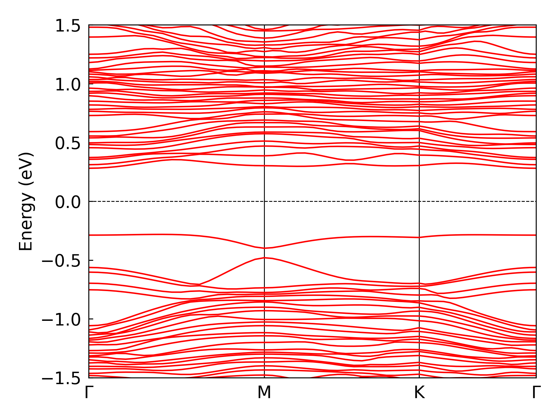
where Emin and Emax set the energy bounds for the band structure plot. The obtained band structure plot is shown in the figure below:
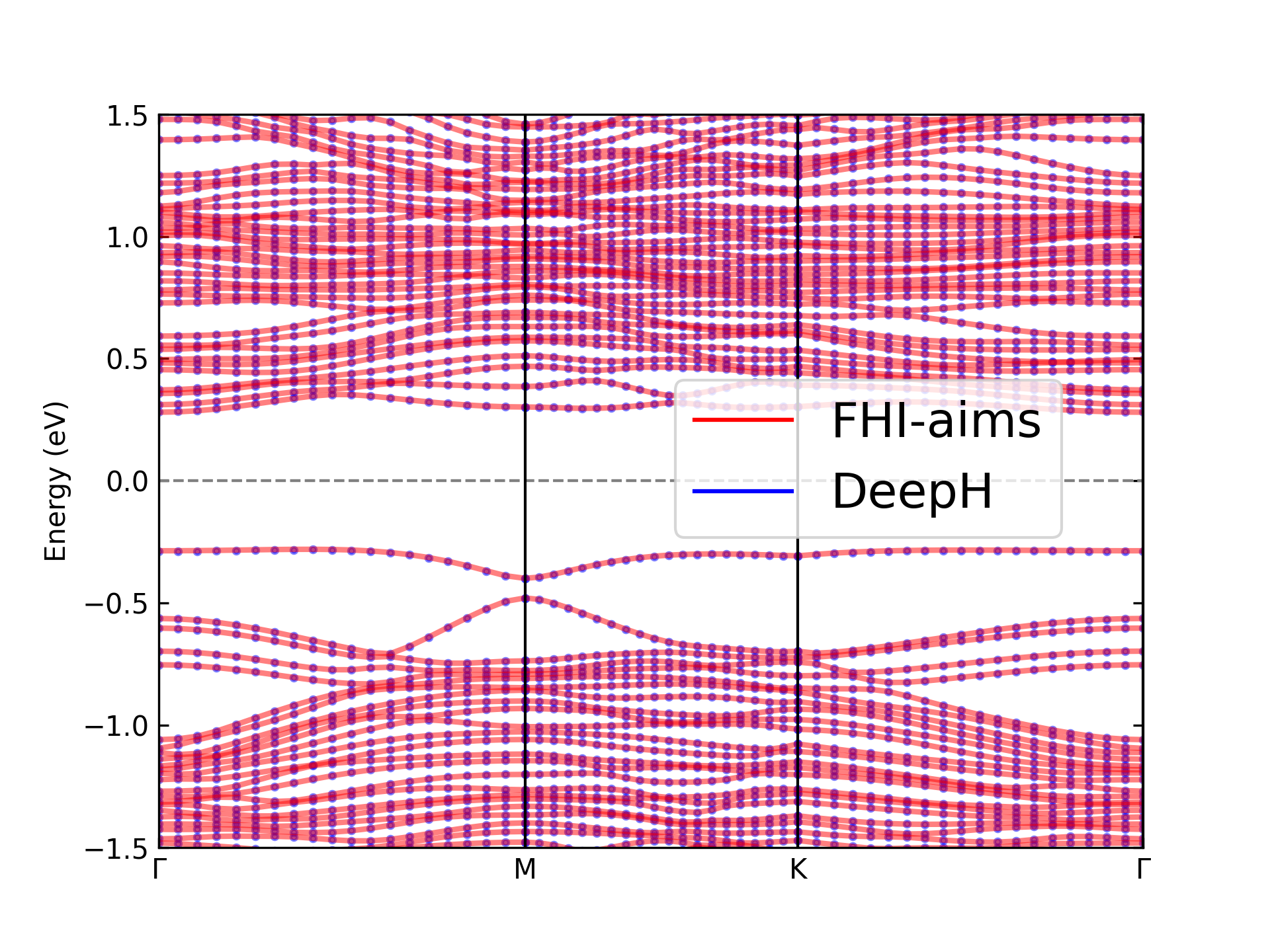
After performing the same processing steps on both the predicted Hamiltonian by DeepH and the Hamiltonian calculated by FHI-aims, and then combining them together, you can obtain the comparison plot as shown below:
Note
The feature enabling direct overlay of FHI-aims band structures onto DeepH results remains under active development, as DeepH-dock is currently in its beta phase.
6. DeepH Accelerates FHI-aims SCF Calculations
As demonstrated above, the Hamiltonians predicted by DeepH are significantly superior to the initial atomic-limit guess Hamiltonians. By feeding DeepH-predicted Hamiltonians back into FHI-aims as restart guesses for continued calculations, the number of SCF iteration steps required for convergence can be dramatically reduced. The corresponding data pipeline is currently under development and will soon be released in the deeph-dock toolkit.